New squelch algorithm for the WebSDR
Pieter-Tjerk de Boer, PA3FWM web@pa3fwm.nl(This is an adapted version of part of an article I wrote for the Dutch amateur radio magazine Electron, January 2018.)
For the WebSDR I recently developed a new squelch algorithm, which in practice doesn't need a manually set threshold. This squelch looks at the signal in the frequency domain.
 See the figure.
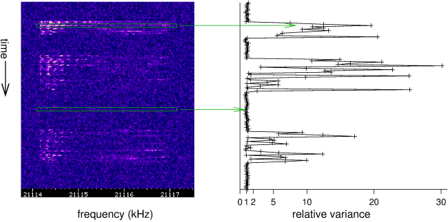
At the left, we see part of a waterfall diagram, in which occasionally a
USB signal is present (someone calling CQ contest, in this case).
We immediately recognize the moments at which the signal is there,
because those are brighter: there is more power, which principle (1) of the previous page uses.
We also see that during the transmissions the audio frequencies between 200 and 600 Hz
are most prominent (this is a USB signal on 21114 kHz, so those frequencies land between 21114.2 and 21114.6 kHz),
which principle (4) uses.
But what is also clear is that when there's no transmission, all pixels on a line are
approximately equally bright (dark blue in this case), while during the transmissions
there are large differences (from dark blue to white).
My idea is to use this: if the differences are small, the squelch must close, and it must open otherwise.
This general idea still needs to be translated into an algorithm that can be programmed in a computer.
See the figure.
At the left, we see part of a waterfall diagram, in which occasionally a
USB signal is present (someone calling CQ contest, in this case).
We immediately recognize the moments at which the signal is there,
because those are brighter: there is more power, which principle (1) of the previous page uses.
We also see that during the transmissions the audio frequencies between 200 and 600 Hz
are most prominent (this is a USB signal on 21114 kHz, so those frequencies land between 21114.2 and 21114.6 kHz),
which principle (4) uses.
But what is also clear is that when there's no transmission, all pixels on a line are
approximately equally bright (dark blue in this case), while during the transmissions
there are large differences (from dark blue to white).
My idea is to use this: if the differences are small, the squelch must close, and it must open otherwise.
This general idea still needs to be translated into an algorithm that can be programmed in a computer.
To measure the amount of variation in the spectrum, we'll use a quantity which I'll call the relative variance: this is the variance divided by the square of the average. It's a number that indicates how much a set of measurement values are spread out, but relative with respect to their average. Practically, this means that the number only depends on the signal/noise ratio, not on the absolute strength of both signal and noise. So we'll repeatedly take one horizontal row from the waterfall diagram (i.e., one set of FFT output bins, one line marked in green in the diagram), and compute the relative variance of the brightness of the pixels on that line. The results is shown at the right.
We clearly see that when there is no signal (e.g., at the lower green marking), the relative variance is around 1; but when there is a signal (upper green marking) the relative variance is much larger. So indeed, this idea can work: the relative variance is a suitable number to base a squelch decision on. Now we still have to choose a threshold: how large must the relative variance be to open the squelch?
| no signal | signal | |
|---|---|---|
| squelch closed | good | error of second kind |
| squelch open | error of first kind | good |
Consider the above table. We see there are four possibilities: there is no signal and the squelch is closed (good!), there is a signal and the squelch opens (also good!), there is no signal but the squelch does open (annoying, an error of the first kind), and finally there is a signal, but the squelch does not open (also annoying, error of the second kind). Of course we want to minimize the likelihood of both kinds of error. However, the choice of the squelch threshold is a compromise. If we set it very high, then the squelch will only open on very strong signals; we'll rarely have errors of the first kind, but many of the second kind. And it's the other way around if we choose the threshold too low.
 Now the nice thing is that we can calculate the probability of errors of the first kind
(the undesired opening of the squelch).
To start, we need to realise that the relative variance is a random number.
We already saw that in the first figure: in the absence of signal, the relative variance
is not exactly 1 every time, but close to it.
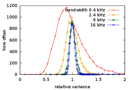
This illustrated more in the adjacent figure.
For this I measured the relative variance more than 9000 times, every time using about a tenth of a second
of pure radio noise, and with different receiver bandwidth settings.
Next, I counted (well, I let the computer count) how often the relative variance had which value.
We see that the relative variance everytime ends up near 1, but the spread around 1 clearly depends on the
receiver bandwidth: more spreading at narrower bandwidth.
Now the nice thing is that we can calculate the probability of errors of the first kind
(the undesired opening of the squelch).
To start, we need to realise that the relative variance is a random number.
We already saw that in the first figure: in the absence of signal, the relative variance
is not exactly 1 every time, but close to it.
This illustrated more in the adjacent figure.
For this I measured the relative variance more than 9000 times, every time using about a tenth of a second
of pure radio noise, and with different receiver bandwidth settings.
Next, I counted (well, I let the computer count) how often the relative variance had which value.
We see that the relative variance everytime ends up near 1, but the spread around 1 clearly depends on the
receiver bandwidth: more spreading at narrower bandwidth.
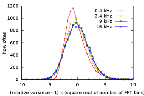 The next picture show the same data, but now I subtracted 1 from the relative variances,
so they are around 0 instead of 1,
and then multiplied them by the square root of the bandwidth (actually: of the number of FFT bins).
We see that the latter step (a "scaling") makes the distributions almost equally wide,
independent of the receiver bandwidth.
So if we use this "scaled" relative variance, the threshold does not need to depend on the bandwidth.
The next picture show the same data, but now I subtracted 1 from the relative variances,
so they are around 0 instead of 1,
and then multiplied them by the square root of the bandwidth (actually: of the number of FFT bins).
We see that the latter step (a "scaling") makes the distributions almost equally wide,
independent of the receiver bandwidth.
So if we use this "scaled" relative variance, the threshold does not need to depend on the bandwidth.
Suppose we set the threshold to 5 and receive only noise, how often will the squelch than open (error of the first kind)? From the 9176 measurements with the 6 kHz filter, 93 exceeded 5 (after scaling), that is about 1%. A 1 percent probability of the squelch opening may seem small enough, but one should realize that this test will be done about 10 times per second: so that 1% means that the squelch will annoy us by opening about once every 10 seconds. That's too often.
With even more data, not from a real receiver but simulated in the computer, we can also check how high the threshold must be to make that probability even smaller. We find that a threshold of 9 is exceeded in 0.1% of cases, 13 in 0.01% and 18 in 0.001%. So we now have a solid basis to control our probability of errors of the first kind: if we set the threshold to 18, the squelch will theoretically open inappropriately only once every 3 hours. That's quite acceptable. In the WebSDR I use two thresholds: 18 for opening the squelch immediately, and 5 with the extra criterion that it needs to be exceeded several times in a row before the squelch opens (e.g. 3 times; the probability of that happening with pure noise is 1% of 1% of 1%, i.e., 0.0001 %).
So we can choose the threshold to make the probability of errors of the first kind acceptably low. But what does this mean for the probability of errors of the second kind, i.e., the probability that the squelch does not open when there is in fact a signal? That probability cannot be calculated easily, because it is of course highly dependent on the strength of that signal. But in practice it turns out that with the threshold choice discussed above, errors of the second kind do not happen a lot: in my experience the squelch already opens on signals that are just too weak to be copied.
Note how useful mathematical statistics is here, even though this is not everyone's favourite topic at school. The fact that the relative variance for pure noise is 1 on average, and the fact that we have to multiply by the square root of the number of FFT bins, can be explained mathematically. And those errors of first and second kind are notions from the field of hypothesis testing: using data (in our case samples of received signals) to draw a well-founded conclusion about whether a hypothesis (in this case "we're receiving pure noise") is true or not.
Text and pictures on this page are copyright 2017, P.T. de Boer, web@pa3fwm.nl .
Republication is only allowed with my explicit permission.