Cable attenuation
Pieter-Tjerk de Boer, PA3FWM web@pa3fwm.nl(This is an adapted version of part of an article I wrote for the Dutch amateur radio magazine Electron, January 2023.)
Cable attenuation
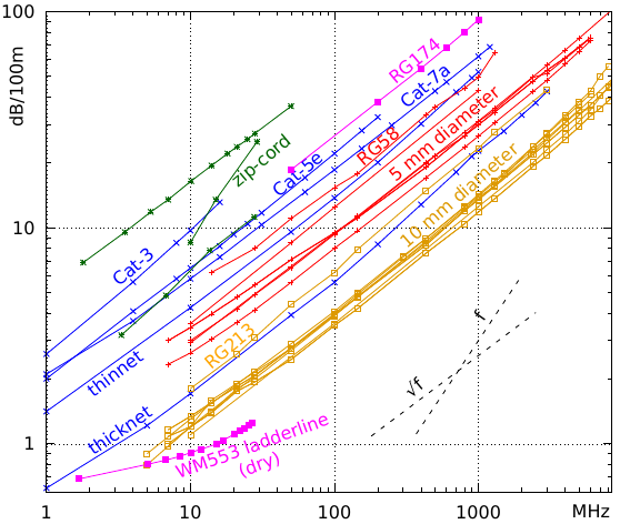 The figure shows the attenuation (also called loss) of various types of cable as a function of frequency.
The blue lines belong to five types of ethernet cable (see the previous part): 'thicknet' (the stiff yellow coaxial cable), 'thinnet' (the flexible coaxial cable), and three types of twisted pair cable: cat-3 for 10 Mbit/s, cat-5e for gigabit, and cat-7a for even higher speeds. We see that the old thicknet cable is actually quite good, comparable to the common RG-213 antenna cable, while thinnet cable is RG58 or similar. The data come from cable manufacturer Belden's website [5], who apparently still can supply thicknet cable!
The red and yellow lines show the attenuation for a large number of coaxial cables of about 5 and 10 mm thickness, respectively, according to data collected by cable supplier Kusch [4]. Particularly the 10 mm thick cables are rather similar, with the exception of the (older) RG213, while among the 5 mm cables the (older) RG58 clearly has more attenuation than the rest. The purple line at the top belongs to the even thinner RG174 coax.
The lower purple line was measured on ladderline [6]. Ladderline consists of two wires spaced by about 1 cm, with some plastic in between, and has an impedance between 300 and 450 ohms. It is notable that the measurement was done when the cable was dry; when wet, the attenuation may be ten times as much [7].
Finally, there are three green lines, showing the attenuation of zip-cord as used for mains power cables, loudspeakers, etc., measured by various radio amateurs [8, 9, 10]. Clearly, they are quite different. Also, the best among these zip-cords is on a par with gigabit twisted pair, at least in terms of attenuation!
Slope
A striking feature of the figure is that the lines are (approximately) straight and almost all are parallel, i.e., have the same slope. Because both axes are logarithmic, a straight line having this slope means that the attenuation increases with the square root of the frequency. E.g., consider the bunch of yellow lines: at 10 MHz their attenuation is a bit above 1 dB per 100 m, and at 1000 MHz it's a bit above 10 dB per 100 m: at a 100 times higher frequency, the attenuation is √100 = 10 times larger.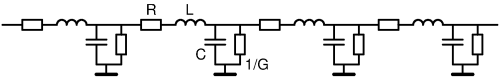
To understand this square-root behaviour, we need to have a look at the equivalent schematic of a transmission line (see also [12]). In this equivalent schematic there are two causes of loss (attenuation): the series resistors R, and the resistors 1/G to ground.
The series resistors R represent the resistance of the metal, usually copper. At higher frequencies this increases due to the 'skin effect': the higher the frequency, the more the current flows only in the outer layer of the conductor. The thickness of this layer is inversely proportional to the square root of the frequency; thus, R increases with the square root of the frequency.
The parallel resistors 1/G represent the losses in the dielectric, the isolation material between center conductor and shield. It turns out that most dielectrics have a 'loss tangent' that is approximately independent of frequency. The loss tangent of a capacitor is the ratio between the AC current running through the (ideal) capacitor C itself, and through its (virtual) loss resistance 1/G. The current in a capacitor increases linearly in frequency, so the (loss) current through 1/G does so too.
In short, the copper losses increase with the square root of the frequency, and the dielectric losses are directly proportional to frequency. Therefore, the total losses are modeled using the formula k1√f + k2f, where f is the frequency, and k1 and k2 are two numbers that depend on the type of cable; k1 for the copper losses and k2 for the dielectric losses. The graph shows that almost all lines have the √f slope far into the GHz range, so apparently the copper losses are dominant.
However, one of the zip-cord lines is clearly steeper than the others, namely approximately linear in frequency rather than its square root. Apparently, the dielectric losses dominate, but only in this type of zip-cord.
Finally, consider the ladderline. First of all, its attenuation is rather low. The wire in WM553 is 1 mm thick, which is thinner than the center conductor of most coaxial cables. Despite this, its losses are lower. That is caused by the higher impedance. The copper resistance forms a voltage divider with the terminating resistance; so the larger the latter is, the lower the losses.
It is also notable that the WM553 line is less steep at lower frequencies. This is because the wire in this type of ladderline is not pure copper, but steel with a layer of copper on the outside: 'copper clad steel'. At higher frequencies the skin effect ensures that the current is running almost exclusively in the copper outer layer. But at lower frequencies the skin depth increases, so part of the current runs in the steel, which has a higher resistance. As a consequence, the losses decrease less at lower frequencies than one would expect based on square-root of frequency.
References
[4] https://kabel-kusch.de/Koaxkabel/Vergleichstabellen.htm[5] https://www.belden.com/products
[6] https://www.kn5l.net/wm553/
[7] Wes Stewart, N7WS: Balanced Transmission Lines in Current Amateur Practice, 1999; https://users.triconet.org/wesandlinda/ladder_line.pdf
[8] https://www.qsl.net/kp4md/zipcord.htm
[9] Jerry Hall, K1TD: Zip-Cord Antennas - Do They Work? QST 3/1979.
[10] https://sites.google.com/site/kr8lus/home/legacy-pages/zip-cord-antennas
[12] Technische notities van PA3FWM, Electron 11/2021; translated online.
Text and pictures on this page are copyright 2023, P.T. de Boer, web@pa3fwm.nl .
Republication is only allowed with my explicit permission.